Auditory-Based Processing of Communication Sounds/Compressive Auditory Filtering

From CNBH Acoustic Scale Wiki

< Auditory-Based Processing of Communication Sounds

Jump to: navigation, search

Thomas C. Walters

This page is currently under construction.
You can check the latest changes in the history.

So far, this thesis has studied the properties of the human auditory system in gradually increasing levels of detail. At the largest scale, the feature representation developed in chapter 2 aimed to emulate the observed behaviour of the system as a scale-invariant preprocessor, which can provide a representation of pulse-resonance communication sounds independent of the pulse rate and the resonance scale of the sound.

'Zooming in' to look at another level of detail, in chapter 3 the process of strobed temporal integration was investigated and placed on firmer theoretical ground. In doing this, it was hypothesised that the auditory images generated using strobed temporal integration should be more robust to noise than features generated from more simple, purely spectral models. This hypothesis was investigated in chapter 4 by adapting the auditory features developed in chapter 2.

Having modelled and observed the large-scale behaviour of the auditory system, and then developed a particular model of the post-cochlear neural processing, this chapter 'zooms in' again to look in finer detail at the behaviour of the cochlea, and in particular its response at very short timescales. The cochlea is perhaps one of the more well-understood components of the auditory system, and there is a wealth of data on the spectral shape of the human auditory filter, and the fine-timing properties of the mammalian cochlea.

The dynamic range of audio signals is orders of magnitude larger than the dynamic range available to encode those signals in the auditory nerve. This means that the auditory system has to perform some sort of compression on the incoming signal in order to represent it effectively with a neural code. It is perhaps surprising to find that the auditory system performs this compression within the auditory filter itself; it uses mechanical feedback from the outer hair cells (OHCs) to dynamically modify the motion of the basilar membrane, and so the signal encoded by the inner hair cells. One important advantage of this approach is that it makes it possible to perform the dynamic range compression with an extremely fast time-constant. The auditory filter is able to compress the peaks of the waveform within a single cycle, and leave the zero-crossings effectively unchanged.

Models of auditory filtering attempt to describe mathematically the processing performed by the cochlea on an incoming sound, which ultimately leads to a neural response. They are a mathematical abstraction of the response of the complex physiological systems in the cochlea to stimulation by an incoming pressure wave. There exist a number of excellent descriptions of various parts of the history of these models, for example Lyon (1996) and Patterson et al. (2003). The introduction to this chapter briefly covers the major points of the various models, and introduces a set of increasingly more complex criteria that an auditory model must fulfil in order to accurately model the human auditory system.

An important feature of the more recent models of the auditory filter is their ability to deal with dynamic compression performed by the cochlea. In this chapter, two recent models of the auditory filter that perform dynamic compression are discussed and analysed. The models are the dynamic, compressive gammachirp (dcGC) (Irino and Patterson, 2006; Irino, Walters and Patterson, 2007) and the pole-zero filter cascade (PZFC) (Lyon et al., 2010). The two filter models are compared in their response to a number of test stimuli to assess the response of the dynamic, time-varying compression that they both implement.

The studies presented in this chapter provide some evidence that dynamic, within-cycle, compression is a feature of auditory processing which is important for correctly modelling human perception of certain stimuli. The stimuli used in this chapter are iterated rippled noise (IRN) and high-pass filtered harmonic complexes in which the fundamental and lower harmonics of the stimulus are not present. These stimuli illustrate well the ability of the auditory system to process temporal regularity in a signal despite the lack of a strong fundamental harmonic, and thus provide a good test for temporal models of audition.

This chapter does not directly address the problem of whether compressive filtering is a crucial element for a good machine-hearing system, but rather looks at the application of compressive filtering to a particular class of stimuli, the correct representation of which is required in a system which accurately models human auditory perception. This is an incremental step towards understanding exactly which aspects of human auditory processing are necessary for effective machine hearing.

A short history of models of auditory filtering

The presence of a set of simple damped resonances, or filters, in the cochlea was conjectured by von Helmholtz (1875), but the idea of resonances in the human auditory system had been discussed as early as 1605 (Wever, 1949). Fletcher (1940) suggested that the peripheral auditory system could be modelled as a bank of bandpass filters with overlapping passbands, on the basis of his measurements of the threshold for detection of a sinusoid when masked by a bandpass noise with a controlled bandwidth. Descriptions of the response of the auditory filter in the frequency domain, based on the results of tone-in-noise masking experiments, came to be known as the `power-spectrum model of masking' Moore (1995). Power spectrum models deal only with stimuli that are static in time, and which only describe the shape of the magnitude spectrum of the auditory filter in the frequency domain; however, this is enough to quantify the overall shape of the filter's transfer function.

The cochlea is known to have a degree of nonlinearity. The fact that the bandwidth of auditory filters exhibits level-dependence, and the presence of distortion products (Kim et al., 1980), particularly in otoacoustic emissions (Moore, 2003), suggests that there is some sort of 'instantaneous nonlinearity' in addition to an overall compression function (Lyon et al., 2010). Another effect that a cochlear model should be able to account for is two-tone suppression (Moore, 2003; Sachs and Kiang, 1968), where an off-frequency stimulus can cause suppression of the on-frequency response of an auditory neuron. Although the effect was first measured in neurons, there is strong evidence to suggest that it occurs in the cochlea (Rhode and Robles, 1974; Rhode and Cooper, 1993; Ruggero et al., 1992).

A set of desirable properties of a practical auditory filter are set out by Lyon et al. (2010). The list is as follows:

Simplicity of description. Either in the time domain, the frequency domain or in the Laplace domain.
Bandwidth control. Filter bandwidth varies as a function of cochlear place, and of sound level.
Realistic and controllable relationship between peak shape and skirts. After bandwidth, the shape of the filter near the edges of its band is the next most important feature, and this should vary with level.
Filter shape asymmetry.
Gain variation. Gain, as well as bandwidth, varies as a function of level.
Stable low-frequency tail. In order to provide a good match to physiological data, the gain of the low-frequency tail of the filter should not vary much as a function of input level.
Ease of implementation as digital filters. In order to make a good digital filter, the model either needs to be described in terms of poles and zeros, be convertible to such a description, or be approximated by such a description.
Connection to the underlying assumptions about the travelling-wave hydrodynamics of the cochlea.
Good impulse-response timing and phase characteristics: for comparison with physiological measurements, across a range of levels, details such as zero-crossing times can be diagnostic of whether the model is faithful to the mechanics.
Dynamic. In addition to being parameterised by level, the filter should be dynamically variable with a fast time constant, such that the filter can compress the glottal pulses in a pulse-resonance sound.

The auditory models set out below attempt to characterise temporal and spectral characteristics of the auditory filter with varying degrees of fidelity, in order to explain the psychophysical data available on masking, compression and two-tone suppression, and electrophysiological data available on the temporal characteristics of auditory filters.

Roex filters for frequency-domain fits

Early efforts to quantify the shape of the auditory filter in the frequency domain employed the `roex' ('rounded exponential') function to describe data from notched-noise masking experiments in humans (Patterson et al., 1982). While the magnitude of the basic roex has a simple description in the frequency domain (a pair of back-to-back exponentials with a rounded top), the phase response is not defined. This in turn leaves the impulse response undefined and so the roex, like other simple descriptions of the frequency spectrum of an auditory filter, cannot be used to make a time-domain filterbank (Patterson et al., 2003). The initial versions of the roex filter, the $roex(p)$ and $roex(p, r)$ were symmetrical in their frequency response, with the latter adding a second parameter to control the shape of the skirts of the filter. The $roex(p u, p l, r)$ added independent control of the parameters for the upper and lower sides of the filter in order to take into account the known asymmetry in filter shape, and the $roex(p, w, t)$ also added asymmetry. Various more complicated versions of the filter emerged, with up to six free parameters. In this way, the roex family could be used to fit human masking data very accurately, but at the expense of adding many additional free parameters.

The gammatone family

In the time domain, the gammatone function had been used for many years to model various forms of auditory response. The gammatone is defined in terms of a gamma-distribution ( $A t n - 1 exp( - b t)$ ) multiplied by a sinusoidal tone ( $cos(ω r t + ψ)$ ), and was first used as a model of basilar membrane displacement by Flanagan and Guttman (1960). The function was reintroduced by Johannesma (1972), who used it to characterise the response of the cochlear nucleus, and by de Boer (1975) to describe the cochlear impulse response measured in cats. The term 'gammatone' was first used to describe the function in 1980 by Aertsen and Johannesma (1980). Schofield (1985) demonstrated that the magnitude response of the gammatone could be used to explain human masking data, and Patterson et al. (1988) then highlighted the similarities between the gammatone magnitude response and the shape of the roex function. Thus the gammatone came to be accepted as a model of the human auditory filter, in both the time domain and the frequency domain.

Since the gammatone had a well-defined impulse response, producing systems to model auditory filters was now possible. Martin Cooke produced an early gammatone filterbank while working with Schofield at the National Physical Laboratory (Cooke, 1993), and John Holdsworth produced the Cambridge gammatone filterbank code while working with Roy Patterson. Practical implementations of the gammatone filter exist both as IIR and FIR filterbanks, and many people use the IIR implementation of Slaney which has the attraction of an accompanying Mathematica workbook (Slaney, 1993). Holdsworth's filterbank code was used successfully over many years as the filterbank in AIM (Patterson et al., 1995).

In its simplest form, however, the gammatone filter is linear, and has a near-symmetrical frequency response around its centre frequency. These properties mean that alone it cannot simulate either the compressive behaviour exhibited by the cochlea, or the asymmetry seen in the auditory filter at high input levels.

Figure 1 – Impulse responses of a gammatone filter (solid line) and a gammachirp filter (dotted line). The chirp parameter,

c

, is

0

for the gammatone and

- 2.0

for the gammachirp

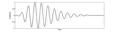
To extend the gammatone, Irino and Patterson (1997) derived the gammachirp filter as the minimum-uncertainty operator for a joint time-scale representation of signals (Cohen, 1993). The derivation is analogous to that of the Gabor function as the minimum-uncertainty operator for a joint time-frequency representation. This is a very deep result, and reinforces the underlying importance of scale in the auditory system. In practice, the gammachirp extends the gammatone by adding a parameter, c, which controls the addition of a log-time term to the carrier ( $cos(ω r t + ψ + c log(t))$ ). This has the effect of making the filter 'chirp' in frequency as a function of time, and adds an asymmetry to the frequency response of the filter. Figure 1 shows the impulse responses of the gammatone and gammachirp filters. The compressive gammachirp (cGC) was first used to fit the simultaneous masking data of Rosen and Baker (1994) and subsets of the masking data from Lutfi and Patterson (1984) and Moore et al. (1990), with the parameter $c$ being allowed to vary as a function of level. They found that it was possible to achieve a similar fit to the masking data with a 4-parameter cGC model as could be achieved with a 6-parameter roex model. Furthermore, the cGC has a well-defined impulse response that can be used to construct a time-domain auditory filterbank.

In practical terms, the cGC can be implemented as a gammachirp filter with an arbitrary value of the chirp parameter, $c$ , cascaded with an `asymmetry function', which is either high-pass or low-pass, depending on $c$ (Patterson et al., 2003). This means in practice that the passive gammachirp filter can be reduced to a static gammatone filter (a gammachirp with $c = 0$ ) and a lowpass asymmetry function. The addition of a complementary high-pass asymmetry function in which centre frequency varies as a function of level allows for a practical cGC filter. Furthermore, the asymmetry functions can be implemented as IIR filters, allowing for an efficient implementation of the filterbank (Unoki et al., 2001).

The dynamic compressive gammachirp filterbank (dcGC) of Irino and Patterson (2006) is a direct descendant of the cGC filter, which models the compressive nonlinearities in the human auditory system. The dcGC is based on the compressive gammachirp (cGC) filterbank Patterson et al. (2003). The dcGC filterbank includes a system for dynamic modification of the cGC filterbank compression parameters in response to the input audio.

Simple representations of the gammatone family in the Laplace domain

Lyon (1997) noted that the representation of the gammatone filter could be simplified by discarding the zeros from the S-plane transfer function to yield an 'all-pole' gammatone filter (APGF). The APGF has fewer parameters than the equivalent gammatone, and has a more controlled behaviour in the tail of the filter. Allowing one zero back into the APGF transfer function yields the one-zero gammatone filter (OZGF); the zero is constrained to lie along the real axis. The special case where the OZGF has its zero at the origin in the S-plane is known as the differentiated all-pole gammatone filter (DAPGF). This extra zero allows more control over the tail of the function than is possible with the standard gammatone function. Furthermore, it provides a simpler way to model the level-dependent gain, bandwidth, asymmetry and centre-frequency shift exhibited by human auditory filters.

Filter cascade models

When considering the analogy between the cochlea and auditory filterbanks, it is important to remember that the cochlea is in fact a complex hydrodynamic system, in which a wave travels along a continuous medium from base to apex. The mechanical properties of the basilar membrane (BM) vary from the basal end to the apical end, and the response of the BM to different frequencies along its length is largely determined by this change (von Békésy, 1960; Moore, 2003). Transmission-line, and more recently, filter cascade models of the cochlea attempt to capture this continuous structure, and describe it as a cascaded sequence of filters. Zweig et al. (1976) used the WKB approximation<ref>The Wentzel–Kramers–Brillouin (WKB) approximation is a technique for approximating the solution of a wave equation, which was originally developed in quantum mechanics. For a wave equation $W (x, t) = A exp(i (k x - ω t))$ , the WKB approximation states that 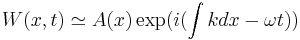$W(x,t)\simeq A(x)\exp(i(\int k dx-\omega t))$ . When k is independent of x, the solution is exact, and as long as k varies only slowly with x, the approximation remains valid. This is equivalent to modelling the slowly-varying properties of the cochlea as a series of discrete filters. See Lyon and Mead (1988) for a complete treatment of the mathematics.</ref> to show that small segments of the cochlea can be seen to act as local filters on the waves propagating down its length, and so it is possible to describe the continuous cochlea as a set of cascaded filters. This led the way for a set of cochlear models known as 'cascade filterbanks' (Lyon, 1998) in which the continuous BM is modelled as a chain of discrete filters with output 'taps' between successive stages (Lyon, 1998).

Such models can provide an efficient method of simulating cochlear dynamics. For example, in a simple fourth-order all-pole gammatone filterbank, each auditory filter is modelled by a cascade of four identical pole-pair filters. A filter cascade has the same architecture, but the stages are non-identical and there is an output at each step. Thus the equivalent cascade architecture would contain only one quarter the number of filter stages as the parallel architecture, for a given number of output channels. This simplicity makes the design an excellent choice for implementation in analogue electronics, and indeed Lyon and Mead (1988) designed an analogue VLSI chip in which each stage was an order-1 (2-pole) APGF.

Lyon (1998) discussed a set of four different transfer functions as possible stages for a filter cascade model of the cochlea. The simplest of these was the 2-pole function. Extra sharpness can be given to the individual filter stages by adding either extra poles or extra zeros to the transfer function. Lyon also presented a three-pole system, and a pair of two-pole, two-zero filters. The sharper of these two-pole, two-zero filters places the pole and zero close to each other and near, but not on, the imaginary axis of the S-plane.

The pole-zero filter cascade

The pole-zero filter cascade (PZFC) (Lyon et al., 2010) is a cascade filterbank in which each stage is described in the Laplace domain by a complex-conjugate pole pair and a similar conjugate zero pair. The stage frequency response is closest to the 'sharper' two-pole, two-zero configuration presented in Lyon (1998). The PZFC frequency response consists of a peak due to the pole, which can be varied by changing the pole quality factor, $Q$ , and a dip caused by the zero. The zero is placed close to the pole on the high-frequency side to give a steep drop in the response above peak frequency. When these segments are cascaded, this approximates the sharp high-frequency cutoff on the auditory filter. The pole $Q$ , or equivalently the pole damping $ξ$ , is varied dynamically to modify the filterbank properties. The filterbank consists of a cascade of these two-pole, two-zero stages and a dynamic smoothing network, as shown in Figure 2. This network takes the output of all the channels, and allows the output of each channel to propagate out over time to affect the pole positions for stages of the filterbank. This dynamic smoothing network allows the filterbank to adapt rapidly to changes in input level and spectral content.

Figure 2 – Cascade structure and smoothing network for the PZFC.

The various parameters of the PZFC can be chosen to give the best fit to various pieces of physiological and psychophysical data. These fits are presented in a later section, but throughout this section I will refer to the 'baseline' parameters, which are the parameters used before fitting. This is the parameter set used in the experiments described in section 2 of chapter 4.

The PZFC was developed by Dick Lyon, based on his previous work on cascade filterbanks. I developed versions of the PZFC filterbank for AIM-MAT and AIM-C, based on Lyon's original implementation.

Pole and zero positions

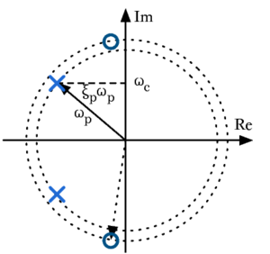
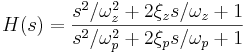
Figure 3 – Diagrammatic representation of the placement of the poles and zeros in the S-plane for the PZFC. The dotted circles show the trajectory of the pole and zero motion as a function of the damping parameter

ξ

.

The pole and zero positions are specified in terms of their natural frequencies ( $ω p$ and $ω z$ , for the pole and zero, respectively) and their damping constants ( $ξ p$ and $ξ z$ ). As the damping is increased from zero, the pole and zero move on a circle in the S-plane. Figure 3 shows the conjugate pole and zero pair; $ω p$ is the natural frequency of the pole, $ω c$ is the instantaneous centre frequency for a given damping, and $ξ p ω p$ gives the pole attenuation (distance from the imaginary axis). The system is described by the following transfer function:

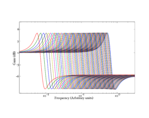
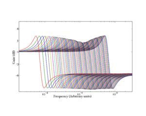
$H(s) = \frac{s^2/\omega_z^2 + 2\xi_z s/\omega_z + 1}{s^2/\omega_p^2 + 2\xi_p s/\omega_p + 1}$

The natural frequencies of the pole and the zero are constants, decreasing from one stage to the next, along a cochlear frequency–place map, or ERB-rate scale. At each stage $ω z$ is fixed at $f_z \times \omega_p$ , where $f z$ is the 'z factor', and is set at 1.4 in the baseline case. The channel density for the filterbank is set by a step factor, which determines the channel density as number of channels per ERB. The channel density is set at 3 channels per ERB in the baseline case. Figure 4 shows the individual filter stages of the PZFC before any adaptation due to the smoothing network, and Figure 5 shows the overall frequency response of the PZFC filterbank at each output.

Figure 4 – PZFC filterbank stages.

Figure 5 – PZFC filterbank overall response before any level modification due to the AGC network.

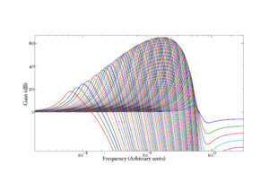
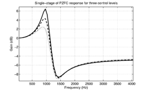
Two parameters, $P damp$ and $Z damp$ , set the damping factors for the pole and the zero respectively. The pole damping varies dynamically as $ξ p = P damp (1 + AGC)$ (where AGC is a function of the state of the automatic gain control circuit described below) and the $Z damp$ parameter sets the zero damping directly: $ξ z = Z damp$ . In the baseline case, $P damp$ is set at 0.12 and $Z damp$ is set at 0.2. Figure 6 shows the effect of changing the two damping parameters on the peak of the stage frequency response.

Figure 6 – Effect of modifying the damping parameters on the PZFC frequency response. When

P damp

is varied,

Z damp

is held at 0.2, and when

Z damp

is varied,

P damp

is held at 0.12.

Automatic gain control

The PZFC automatic gain control (AGC) is achieved by a temporal and spatial smoothing network. This network takes the output of all the channels, applies smoothing in both the time and frequency dimensions, and uses both global and the local averages of the filterbank response to affect the pole damping, $ξ p$ at each stage. In Lyon’s implementation, the dynamic smoothing network allows the filterbank to adapt to changes in the input on time scales from the order of a few milliseconds up to hundreds of milliseconds. While it is useful, in practical terms, to ascribe AGC timescales on the order of hundreds of milliseconds to processes in the cochlea, it is not physiologically realistic. Adaptation that occurs on this timescale is likely to originate more centrally.

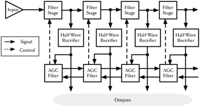
Figure 7 – Impulse response of one of the four sets of parameters in the AGC smoothing network. The activity diffuses out in space and decays exponentially in time.

Figure 8 – PZFC filterbank stage at three different levels

The smoothing network takes the form of a four-stage filtering process. The output of each filter channel is first half-wave rectified and weakly compressed using a cubic nonlinearity. This monopolar signal is then passed through a set of low-pass filters, which have the effect of smoothing the signal. Four first-order filter stages are arranged in parallel, each having one state variable per channel. Each stage has a different time constant, which determines how much the state in a channel should be affected by the current filter output. Spatial smoothing is achieved by coupling the states to their neighbours at adjacent channels --- a simple filter convolves the AGC state for each stage with a three-channel wide triangular window, once per sample. This has the effect of causing the signal in one channel to gradually diffuse out to affect the control parameters in other channels. An application was designed to reveal the spread of adaptation in frequency and time, in preparation for experiments designed to examine the physiological plausibility of the smoothing network, which is unlikely to be symmetric in the cochlea. Figure 7 shows the impulse response of the smoothing network. Note the exponential decay in the centre channel, and the symmetrical diffusion of activity out to more distant channels. Figure 8 shows the response of a single filter stage as the pole position is modified by the AGC system.

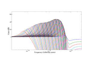
The pole dampings in each channel are scaled (increased from their values in quiet) by a factor proportional to the mean of the four AGC stages in that channel. Thus, a sustained high input level in a channel will cause the poles for the associated filterbank stage, and those around it, to move further from the imaginary axis in the S-plane, reducing the gain and sharpness of the combined filter in that channel and those around it. As time passes, this damping effect will propagate to more distant channels, until an equilibrium state is reached. Figure 9 shows the response of the individual filter stages after adaptation to a human /a/ vowel, and Figure 10 shows the overall filterbank response after adaptation. The original response of the filter stages, before adaptation, is seen in Figure 4.

Figure 9 – PZFC filterbank stages after processing several seconds of audio. The AGC network has caused the response of the individual stages to change.

Figure 10 – Overall PZFC filterbank response after processing several seconds of audio.

The smoothing network is intended to simulate the active mechanism in the cochlea, whereby the outer hair cells (OHCs) dynamically modify the response of the basilar membrane to a stimulus. The cascade architecture of the PZFC mimics transmission-line architecture of the cochlea, in which the incoming wave travels along a medium with slowly-changing properties. This makes the filterbank a more physiologically plausible model of the processing actually occurring in the cochlea. However, as it stands, the AGC mechanism does not model the physiological system particularly accurately. There is currently no known physiological analogue for a mechanism by which gain control information propagates symmetrically out from a point on the basilar membrane to points both higher and lower in frequency.

Fitting the PZFC to human masking data

Two studies, by Baker et al. (1998) and Glasberg and Moore (2000), measured the threshold in humans for detection of a sinusoid in asymmetric notched noise. Both studies covered a large range of frequencies and levels, spanning most of the normal range of hearing. The data from these studies were used by Patterson et al. (2003) to fit a set of parameters for the cGC filter; they describe a fitting technique for auditory filters, based on the 'polyfit' procedure which was used by Baker et al. to fit roex functions to their original data.

The polyfit procedure attempts to fit a frequency-domain auditory filter to a set of masking data obtained with a single probe frequency at a wide range of probe levels. Patterson et al. (2003) extended the technique to allow fitting to data from multiple probe frequencies simultaneously. The updated procedure makes the assumption that the variation of any of the filter parameters with probe frequency can be represented as a linear function of the frequency in ERBs.

Figure 11 – Results of a fit of human masking data to a PZFC with 10 free parameters. (Fit 517 from Figure 12). Panel (a) shows the absolute frequency response of the filters as a function of stimulus level. Panel (b) shows the responses at a single stimulus level with the filter tail tied at 0dB gain. Panel (c) shows the equivalent rectangular bandwidth of the filter (ERB) as a function of centre frequency, for three different probe levels. Panel (d) shows the input-output curve for the filterbank as a function of level. In this panel, the dotted line shows a linear response, and the red lines correspond to the different filter centre frequencies.

In the case of the gammachirp filter, the procedure fits a total of five filter parameters with constants or linear functions. The total number of free parameters used for the filterbank can be set by choosing how many of the filter parameters to represent as constants, and how many as linear functions. A further two non-filter parameters are fitted with parabolic functions, rather than linear functions. These non-filter parameters, $K$ and $P 0$ , define the efficiency of the detection mechanism following the cochlear filter, and the lower limit on the threshold respectively.

Lyon used the fitting routines employed by Patterson et al. to fit the PZFC to human masking data. In order to fit the human masking data of Baker et al. and Glasberg and Moore with the PZFC, a number of modifications were made to the fitting technique described by Patterson et al.. K, the measure of detection mechanism efficiency, was removed from the search space as it can be determined from the other parameters. In addition to this, search over centre frequencies was made near-continuous to minimise confusion of estimated gradients, and the robustness in small-signal behaviour was improved.

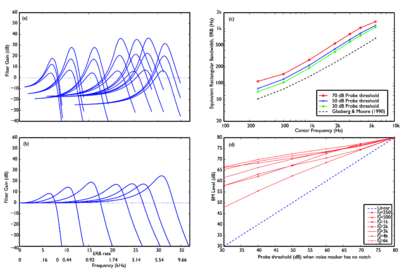
Figure 11 shows the results of fitting the PZFC to the masking data of Baker et al. (1998) and Glasberg and Moore (2000). The four panels show various aspects of the response of the filterbank. The top-left panel shows the absolute frequency response of the filters as a function of stimulus level. The bottom-left panel shows the responses with the filter tail tied at 0dB gain. The filter gain increases in the low ERB range, and levels off in the higher ERB range. The top-right panel shows the equivalent rectangular bandwidth of the filter (ERB) as a function of centre frequency, for three different probe levels. Filter bandwidth is seen to increase as a function of level, but even at the lowest level, the bandwidth is above that estimated with the gammatone. The bottom-right panel shows the input-output curve for the filterbank as a function of level. In this panel, the dotted line shows a linear response, and the red lines correspond to the different filter centre frequencies.

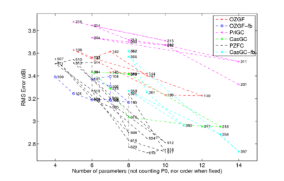
Figure 12 – RMS fitting error as a function of number of parameters, for a number of filter types. This plot was generated using Lyon's updated filter fitting routines. `OZGF' is the one-zero gammatone filterbank and `PrlGC' and `CasGC' are parallel and cascade gammachirp filterbanks respectively. In the `-fb' variants, feedback from the output in a filter channel controls the gain of the filterbank in that channel (a potentially unstable configuration).

Figure 12 shows the RMS fitting error as a function of number of parameters, for a number of filter types. The plot was generated using Lyon's updated filter fitting routines, and it shows that the PZFC can fit the human masking data more accurately with fewer parameters than the parallel and cascade versions of the compressive gammachirp filterbank.

Figure 13 --- Results from fitting the compressive gammachirp filterbank to human masking data. The figure is taken from Unoki et al. (2006). Panel (a) shows the absolute frequency response of the filters as a function of stimulus level. Panel (b) shows the responses of the component filters of the cGC. The solid lines show the response of the passive gammachirp filter, and the dotted lines show the response of the active filter. Panel (c) shows the equivalent rectangular bandwidth of the filter (ERB) as a function of centre frequency, for three different probe levels. Panel (d) shows the input-output curve for the filterbank as a function of level for a range of different centre frequencies,

P g c p

is the output level of the passive gammachirp filter.

Figure 13 shows the characteristics of the compressive gammachirp (cGC) filterbank in the same format as presented in Figure 11 for the PZFC. This allows for comparison of the two filterbank responses in a greater level of detail. The cGC is the filterbank upon which the dynamic compressive gammachirp (dcGC) is based. While the results for the PZFC and the cGC are similar, there are some differences between the responses of the two filterbanks. In panel (a), the cGC is seen to have a steeper high side to the filter. Panel (c) shows the bandwidth as a function of filter centre frequency. In both cases, the filter bandwidths are wider for louder signals, as would be expected, and they both follow the form of the measured ERB function in humans well. However, the PZFC has a smaller range of variation in bandwidth as a function of level. The compression functions (shown in panel (d)) show a smaller spread as a function of frequency in the PZFC compared to the cGC. The PZFC also has a less well-organised structure to the compression functions than the cGC. Overall, the PZFC fits the masking data well using fewer parameters than the dcGC, but the compression functions are not as orderly, and the upper side of the PZFC is probably not quite as sharp as it should be.

The dynamic compressive gammachirp

The dynamic compressive gammachirp (dcGC) filterbank is a parallel-architecture filterbank with a cascaded control channel (Irino and Patterson, 2006).

It was demonstrated by Irino and Unoki (1999) and Unoki et al. (2001) that the gammachirp filter can be decomposed into a cascade of a gammatone filter and an asymmetric compensation function that controls the effective value of the chirp parameter, $c$ . Indeed, the chirp parameter of any gammachirp filter can be modified by cascading it with an asymmetric compensation function of the correct form. Such a cascade architecture is used in the dcGC filterbank to dynamically modify the chirp parameter of each filterbank stage independently as a function of the input signal. Figure 14 shows the response of the passive gammachirp filter, the high-pass asymmetric compensation filter for different levels, and the response of the combined compressive gammachirp (cGC) filter.

Figure 14 --- Response of the passive gammachirp filter (pGC), the high-pass asymmetry function (HP-AF), and the compressive gammachirp (cGC) filter for probe levels of 30, 40, 50, 60, and 70 dB. Figure taken from Irino and Patterson (2006) used with permission of the authors.

In the first, passive, stage, the incoming signal is passed through a gammachirp filterbank that has no level-dependence. In the active part, the output of each channel is passed through a dynamically controlled asymmetric compensation filter that modifies the bandwidth and peak frequency of the overall composite filter. The parameters of this active asymmetric compensation filter are controlled by the processed output of a higher-frequency channel in the filterbank. The control parameter is an estimate of the instantaneous output level of the control channel. This level estimate is calculated from a linear combination of the original passive filter output, and the output of an asymmetric compensation filter with fixed parameters acting on that output.

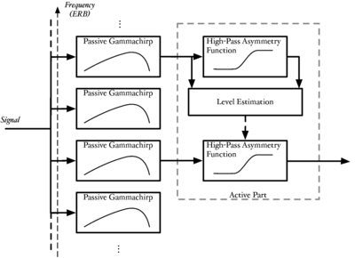
Figure 15 -- Architecture of the dcGC filterbank

Figure 15 shows the architecture of the dcGC. The active part is shown for only one channel of the filterbank. The solid lines show the path of the signal through the filterbank, and the dotted line shows the control parameter for the active high-pass asymmetry function. Since the control parameter is updated instantaneously (on a sample-by-sample basis in the digital implementation), the filterbank exhibits extremely fast-acting compression at sub-millisecond timescales. This compression allows the filterbank to compress the individual glottal cycles in human vocalisations, while allowing the resonance that follows them to ring. Thus the dcGC can effectively reduce the dynamic range of an input signal, and facilitate the analysis of the resonance information following a pulse. The various parameters of the dcGC filterbank have been fitted to human masking data over several studies (Unoki et al., 2001; Irino and Patterson, 2001; Patterson et al., 2003; Irino and Patterson, 2006; Unoki et al., 2006).

Comparing the PZFC and the dcGC

The architecture of the dcGC is fundamentally different from that of the PZFC. Whereas the dcGC is essentially a parallel filterbank wherein all filters get the same input signal, the PZFC is a cascade filterbank with each filter fed by the one before it in the cascade. A further major difference is in the flow of activity in the AGC circuits. In the PZFC, activity from a filter spreads out in both directions symmetrically to influence the response of both lower and higher frequency filters. In the dcGC, the activity in each channel affects only one other channel in the filterbank, as the control signal always flows from a higher-frequency channel to a lower-frequency channel.

The major benefits of the PZFC are that it is efficient to implement, either in hardware or in software (because it consists of a simple cascade of second-order filters) and that it accurately models the travelling wave in the cochlea. By contrast, the dcGC, while still efficient, uses a fourth-order filter cascaded with a set of four second-order asymmetry functions for the signal path in each stage, and another four second-order asymmetry functions for the level estimation path. However, the dcGC has a sound theoretical basis from the point of view of the optimal processing of pulse-resonance sounds; the automatic gain control bears more resemblance to that seen in the cochlea, and it has been well tested in several models. It is for these last two reasons that the PZFC needs more testing and improving before it can be considered as good as the dcGC for modelling auditory processing.

A further problem with the PZFC is that, in the design detailed in this thesis, it is not able to successfully model the data on zero-crossings of the auditory filter response. Studies have shown that the chirp rate of the auditory filter does not vary with the level of the stimulus (Carney et al., 1999), and so the zero-crossings of the impulse response should remain fixed in time as the level changes. However, because the AGC causes the poles of the filter to move in circular trajectories in the S-plane, the zero-crossings of the PZFC impulse response do shift with level. Recently, Lyon (personal communication) has shown that the positions of the zero crossings can be fixed by making the poles move parallel to the real axis, but details of this change are not currently available.

Figure 16 --- `Cochleagrams' of the output of the PZFC, dcGC and gammatone filterbanks for the word `washwater' spoken by a woman. The level in each plot is scaled such that the darkest greyscale value corresponds to the highest output level for each filterbank, and the greyscale level decays from there to zero for pure white. This allows for comparison of the relative dynamic range of each of the filterbanks.

The main benefits of a compressive filterbank come from its ability to actively and quickly compress the pulses in a pulse-resonance sound, and then to recover quickly in order to retain the resonance information that follows. Figure 16 shows 'cochleagrams' for the word 'washwater' after processing through the PZFC, dcGC and gammatone filterbanks. A 'cochleagram' has the same dimensions as the spectrogram, but the output is continuous in each filter channel, unlike the spectrogram where the output is quantised into 'frames' by the window time-step. No external compression was applied to the output of the filterbanks. The dcGC and PZFC filterbanks compress the output into a smaller dynamic range than the simple gammatone filterbank. The dcGC is particularly effective in bringing up the level of the formants relative to the glottal pulses for the voiced sections. However the PZFC is better at enhancing the level of the unvoiced sections, particularity the 'sh' sound between about 200 and 360ms. These effects are likely to be due to the different time constants employed in the gain control circuits of the two filterbanks. The dcGC has very fast-acting compression, but no time constants that are longer than a few milliseconds. This means that it is very effective in compressing the glottal pulses, but it does not have much effect on the longer-term dynamics of the stimulus. The PZFC, by contrast, has AGC time constants up to the order of hundreds of milliseconds, and so is able to affect the relative level of the output on syllable-length timescales. From this, it seems that there may be a trade-off between fast-acting compression and longer-term gain control.

Figure 17 --- `Cochleagrams' of the output of the PZFC, dcGC and gammatone filterbanks for a two-formant synthetic vowel. The level of the stimulus was ramped down linearly (on a dB scale) from a maximum to -48dB over the course of one second. Scaling is as in Figure 16 so that dynamic range can be compared.

Figure 18 --- `Cochleagrams' of the output of the PZFC, dcGC and gammatone filterbanks for a two-formant synthetic vowel. The level of the stimulus was ramped up linearly (on a dB scale) from a minimum of -48dB to the maximum amplitude possible over the course of one second. Scaling is as in Figure 16 so that dynamic range can be compared.

Figure 17 and Figure 18 show the responses of the PZFC, dcGC and gammatone filterbanks to a two-formant synthetic vowel that changes rapidly in level over the course of a second. In both cases, the PZFC compresses the output most strongly, leading to the longest visible patterns of activity in the image.

In the remainder of this section, the detection of periodicity in various stimuli is used to compare the temporal dynamics of the dcGC and the PZFC filterbanks. It seems that dynamic, compressive filterbanks produce better features for modelling pitch strength within time-domain models such as AIM. Specifically, use of the PZFC or the dcGC filterbank within AIM was found to provide a more pronounced peak in the temporal profile of the auditory image than the standard gammatone filterbank, for complex sounds like iterated rippled noise (IRN).

The mechanism that sharpens the peak is not immediately clear, but what is clear is that time-varying compression is an important factor in the processing of these stimuli. In the following sections I detail a number of experiments performed to judge the ability of an AIM-based model with a dcGC or PZFC filterbank to detect the dominant periodicity in these stimuli.

Stimuli

Iterated rippled noise

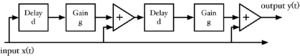
Iterated rippled noise (IRN) is a stimulus that is frequently used as a test of auditory models. It has a power spectrum that resembles that of a noise, but gives rise to a pitch percept in the auditory system. IRN is created by repeatedly time-shifting and summing a block of white noise. This has the effect of adding a repeating temporal structure to the noise. After several iterations of this delay-and-sum process, a weak pitch is observed in the stimulus, which gradually becomes stronger as more iterations are performed. Figure 19 shows a circuit for generating IRN by repeatedly adding a delayed version of the waveform to itself. In the spectral domain, the delay-and-sum process adds a small `ripple' to the spectrum of the sound, which gives it a weak harmonic structure. Repeated iterations of the delay-and-sum process enhance the depth of the ripple.

Figure 19 --- Circuit for generating IRN. Two iterations shown. Figure redrawn from Yost et al. (1996).

The phenomenon of a repeated noise giving rise to a pitch was first reported by Huygens (1693), who observed that a pitch was present in the sound of a fountain opposite a flight of stone steps. Huygens determined that the pitch of the sound was equivalent to that generated by a small organ pipe of the same length as an individual step. The multiple reflections of the fountain noise from the vertical surfaces of the staircase had the effect of summing multiple copies of the noise waveform, giving rise to what we would now call IRN. A similar effect has been observed in Mexican step pyramids, where a handclap elicits a chirping noise reflected from the vertical surfaces (Bilsen, 2006).

IRN is an excellent stimulus for testing the characteristics of filterbanks and strobed temporal integration mechanisms (see chapter 3). IRN has been a challenging stimulus for spectral models of pitch perception (Yost and Hill, 1979). Pitch extraction in AIM is based on the temporal fine structure of a sound, and pitch strength corresponds to the peak height in the temporal profile of the SAI. Thus, the auditory image model gives a specific way of modelling the pitch strength of stimuli which lack a strong spectral structure.

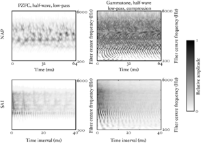
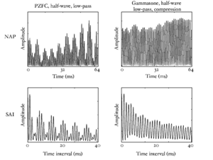
Figure 20 --- NAPs and SAIs generated from a 16-iteration IRN stimulus using the PZFC and gammatone filterbanks. The PZFC output is half-wave rectified and lowpass filtered (hl), the gammatone filterbank output is logarithmically compressed as well as being half-wave rectified and low-pass filtered (hcl).

Figure 21 --- The output of the 770Hz channel in Figure 20

Figure 20 and Figure 21 show the response of the PZFC and gammatone filterbanks to the same IRN stimulus, and the resulting SAIs generated from the signal. The pitch feature in the SAI of the PZFC is better defined than that in the SAI of the simple gammatone filterbank.

Measures of pitch strength

In order to further investigate the pitch strengths produced by the three filterbanks it is necessary to have some absolute measure of pitch strength in the SAI temporal profile. Ives and Patterson (2008) developed just such a measure, which estimates the pitch strength of harmonic complexes from the vertical ridge of activity that appears in the SAI at the time interval associated with the pitch. Their measure was simple: they computed the temporal profile and found the largest peak in the region of the time-interval associated with the pitch. They then found the two local minima immediately adjacent to this peak, and took the mean of the levels of the two minima. This mean minimum level was then subtracted from the level of the maximum to get a local peak height. This was taken as the pitch strength. Ives and Patterson (2008) used this to study the relative pitch strength from a model using the dcGC filterbank and the gammatone filter.

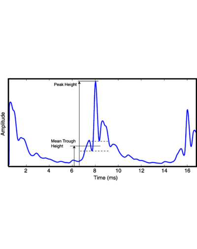
Figure 22 --- Pitch strength measure used by Ives and Patterson (2008). This figure is modelled on figure 6 from Ives and Patterson (2008).

This pitch strength measure was used to estimate pitch strength from the temporal profiles of auditory images. The technique of Ives and Patterson (2008) was modified slightly in two ways. Since the repetition rate of the stimuli was already known, the search space for a local maximum in the SAI temporal profile was limited to a region around the fundamental. The search space for a maximum was 1.5ms each side of the repetition rate. In order to compare the output of different filterbanks, the SAI temporal profiles were all normalised such that the local maximum in the region of the pitch was at 1. Since the SAI profiles were truncated at 0.5ms (the standard parameter for the ti2003 AIM-MAT module), this led in many cases to the peak due to the repetition rate being the highest point in the temporal profile. However, in some cases, particularly for the PZFC, the decay rate in the SAI profile after the zero-lag peak was such that the SAI profile was at a higher value near the zero-lag line. This effect is visible in some panels of Figure 26, where the temporal profile is 'clipped' at the low-lag end. Figure 22 shows how the measure is calculated from the peak and adjacent troughs.

Comparison to human pitch perception

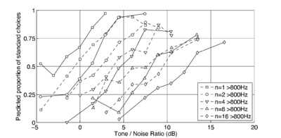
The normalised pitch-strength measured for IRN stimuli was compared with the pitch strength measured for IRN in perceptual experiments. Patterson et al. (1996) performed a series of experiments on the human perception of IRN by comparing the pitch strength of IRN stimuli and tonal stimuli masked with noise (Yost, 1996; Yost et al., 1998; Patterson et al., 2000; Handel and Patterson, 2000). Subjects compared IRN with different numbers of iterations to a tonal stimulus (256-iteration IRN with a 16ms delay time) masked with noise. Subjects were asked to select the stimulus with the stronger pitch strength as the SNR of the noise-masked tonal stimulus was changed. In their experiments two conditions were tested, in which the stimuli were high-pass filtered with a cutoff frequency of either 50Hz or 800Hz. The 800Hz filter condition was designed to exclude the resolved harmonics from the stimulus. The pitch strength measure described above was used to model the data of Patterson et al. (1996), using the techniques described in that study. The original results from the perceptual experiment are plotted in Figure 23, the predictions made by Patterson and Yost's model are shown in figure Figure 24 and the predictions made using the current measure on an SAI made using a PZFC filterbank are plotted in Figure 25. In each case, the horizontal axis is the tone to noise ratio, and the vertical axis is the predicted proportion of the time that the standard noise-masked tonal stimulus was picked as having a higher pitch strength than the IRN stimulus. In practice the results of Patterson et al. (1996) did not show much difference between the 50Hz and 800Hz condition, and a similar result was seen when using the pitch strength measure described here, so only the more challenging 800Hz condition is compared.

Figure 23 --- Psychometric functions for test IRNs from Patterson et al. (1996) (Figure 1).

Figure 24 --- Pitch strength predictions for the perception of IRN in noise, from the autocorrelation model ofPatterson et al. (1996) (Figure 5).

Figure 25 --- Predictions (dashed lines) of the perceptual data of Patterson et al. (1996) (solid lines) made using the normalised pitch strength measure employed in the experiments in this section applied to auditory images generated with a PZFC filterbank. The results follow the same pattern as the perceptual results reported in Patterson et al. (1996), but the measure is slightly noisier than the model used in that paper.

The predictions made by the normalized pitch strength measure in Figure 25 have the same form as the perceptual results reported in Patterson et al. (1996). The form of the results for the other filterbanks is similar. The curves predicted by this model are a little noisier than those from the model of Patterson et al. (1996), but the model has the advantage of being normalised making it easier to compare results across filterbanks when their output levels differ.

Experiments

Comparing pitch strength estimates using IRN

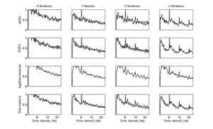
Figure 26 --- SAI temporal profiles generated with four different sets of filterbank / NAP parameters for an IRN stimulus with a delay of 8ms. The leftmost column shows the SAI temporal profile for a zero-iteration IRN, which is a noise. The remaining columns show the response for 1, 2, and 4 iteration IRN stimuli. For the 1, 2 and 4 iteration IRN, a peak is expected in the temporal profile at 8ms time interval.

Figure 26 shows SAI temporal profiles generated with the dcGC, the PZFC and the gammatone filterbank with and without logarithmic compression for IRN stimuli. The profiles for the zero-iteration IRN (just noise) show little temporal structure, as we would expect. It is clear from inspection that the gammatone filterbank with logarithmic compression produces profiles in which the peak in the profile which corresponds to the perceived pitch is much less strong than for the other filterbanks. For comparison, the results from the gammatone filterbank without logarithmic compression are included. The pitch strength estimates are stronger than for the log-compressed gammatone, but the linear gammatone is not a physiologically reasonable auditory filter model as it has no compression, and it is included in these experiments only for comparison with the other compressive filterbanks.

While the dcGC might be considered to give slightly higher pitch strength estimates based on the data in the figure, there is not any clearly visible difference between the PZFC, the dcGC and the linear gammatone models.

Auditory images were generated from IRN stimuli with 0, 1, 2 and 4 iterations, as described above. The IRN stimuli (specifically IRNo, see Yost et al. (1996)) were generated using the `gen\_IRNo' function in AIM-MAT, and were used to assess the effect of overall pitch saliency on the pitch strength measures extracted from the SAI. The IRN was generated with a delay of 8ms, leading to a 125Hz pitch in the output. The output was band pass filtered with a pass band between 500Hz and 2kHz. The pass band was ramped up over 200Hz and down over 1.6kHz using a raised cosine window; therefore the region of the spectrum containing energy went from 300Hz to 3.6kHz. This bandpass filtering serves to remove the fundamental and second harmonic of the pitch period from the spectrum completely.

Results

<tablenameRef name="irn_results_table"/> shows the mean results from application of the pitch strength estimation algorithm to 20 randomly generated IRN stimuli using the above parameters. It is clear from these results that the dcGC gives rise to a considerably stronger pitch feature in the temporal profile of an IRN stimulus than do the other filterbanks. While the pitch feature from the PZFC is stronger than that from the log(gammatone) filterbank, the results are on a par with the results from the linear gammatone. Standard deviations for the pitch strength measures are given in brackets after each value.

<tablename name="irn_results_table"/> Mean pitch strength estimates for 20 randomly-generated IRN stimuli using four filterbanks and 1, 2 and 4 iterations when generating the IRN.
	dcGC	PZFC	log(gammatone)	gammatone
1 Iteration	0.553 (0.055)	0.441 (0.056)	0.297 (0.040)	0.421 (0.044)
2 Iterations	0.566 (0.089)	0.461 (0.056)	0.313 (0.049)	0.432 (0.061)
4 Iterations	0.633 (0.051)	0.504 (0.055)	0.342 (0.058)	0.502 (0.049)

The results suggest that the processing performed by the dcGC is fundamentally different to that performed by the PZFC for these stimuli. In order to determine why performance with the PZFC is inferior to that with the dcGC, we now turn to a deterministic signal to perform several experiments on the AGC of the PZFC.

Harmonic complexes

Clara Suied generated an interesting set of bandpass-filtered harmonic complexes for an experiment on the perception of pitch height. These stimuli were 125Hz harmonic tones, in which the 9th harmonic was the lowest component. The envelope of the amplitude spectrum was flat in a pass band which was six ERBs wide. This is a stimulus design suggested by Krumbholz et al. (2000). Above the flat pass band, the envelope of the amplitude spectrum was smoothly attenuated to zero with a quarter-cycle cosine envelope function. Below the passband, the envelope was simiarly raised from zero with a quarter-cycle sine envelope. The width of the envelope function below the passband was 2 ERBs, and above the passband it was 4 ERBs.

In the experiments below, Suied's baseline stimulus is used to experiment with modifications to the PZFC automatic gain control (AGC). For quantitative measurement of the effect of changes on the PZFC parameters, these stimuli are easier to deal with than IRN because IRN is inherently a noisy stimulus, and it would be necessary to average over stimuli to achieve measurements that can be used for comparison.

Modified PZFC AGC parameters

The base harmonic complex stimulus (0 degrees phase shift, no spectral envelope shift) was used to further assess the effect of changing the PZFC parameters on the pitch strength measures produced with that filterbank.

Temporal smoothing in the PZFC AGC is implemented with a smoothing filter that is convolved with the AGC activity once per sample. The filter is three channels wide and in the default configuration is triangular in form. Choosing the relative levels of the three coefficients changes the way in which energy is distributed in the smoothing process.

The default configuration of the smoothing filter has the coefficients 0.3, 0.4 and 0.3 (left, centre and right). The parameters sum to unity in order to maintain the overall activity within the AGC smoothing network. When these coefficients are convolved with the smoothing network activity in each channel, the activity spreads out equally to higher and lower frequencies. This default configuration is tested as parameter set 0 in the experiments below.

To force the activity to spread asymmetrically, the experiments above were repeated with several different configurations of the AGC parameters. These configurations are designed to be weakly and strongly asymmetrical, preferentially pushing activity either to lower frequencies (as in the dcGC) or to higher frequencies. The configurations of the parameters, along with the pitch strength estimates, are shown in <tablenameRef name="pzfc_agc_coeffs"/> as parameter sets 1 to 6. In the case of parameter sets 5 and 6, the activity does not diffuse along the spatial dimension but is actively 'transported', since one of the off-centre coefficients is larger than the central coefficient.

The AGC also has four temporal constants $ε n$ where $n$ is from 1 to 4. These parameters determine the decay rate of activity in each of the four AGC channels. The activity in the AGC channel is attenuated by a factor of $1 - ε n$ at each time step, and the current activity from the filterbank channel is added with weight $ε n$ . In channels with a large constant, activity in a channel at a certain time dies away quickly. Conversely, a small decay constant leads to activity affecting the AGC state for a longer period of time.

The default decay constants for the PZFC AGC are 0.0064, 0.0016, 0.0004 and 0.0001 per sample. At a sample rate of 44kHz, these constants correspond to activity half-lives of roughly 2ms, 10ms, 40ms and 160ms. These constants can be modified to change the integration time of the AGC.

Several alternative sets of constants were tried to test the temporal dynamics of the filterbank. Since none of the AGC parameters were actually fitted when the PZFC was fitted to the masking data, we are free to choose values which give the best temporal dynamics for the filterbank. The modified AGC coefficients, and pitch strength estimates, are shown in lines 7 to 11 of <tablenameRef name="pzfc_agc_coeffs"/>.

<tablename name="pzfc_agc_coeffs"/> Tested configurations of the PZFC spatial and temporal smoothing filters, and measured pitch strength for a harmonic complex using these parameters. Spatial coefficients are from high frequency to low frequency.
	Spatial	$ε n$	Pitch strength
0	0.3, 0.4, 0.3	0.0064, 0.0016, 0.0004, 0.0001	0.698
1	0.1, 0.5, 0.4	0.0064, 0.0016, 0.0004, 0.0001	0.695
2	0.4, 0.5, 0.1	0.0064, 0.0016, 0.0004, 0.0001	0.702
3	0.0, 0.5, 0.5	0.0064, 0.0016, 0.0004, 0.0001	0.713
4	0.5, 0.5, 0.0	0.0064, 0.0016, 0.0004, 0.0001	0.716
5	0.0, 0.2, 0.8	0.0064, 0.0016, 0.0004, 0.0001	0.777
6	0.8, 0.2, 0.0	0.0064, 0.0016, 0.0004, 0.0001	0.691
7	0.3, 0.4, 0.3	0.0128, 0.0032, 0.0008, 0.0002	0.683
8	0.3, 0.4, 0.3	0.0256, 0.0064, 0.0016, 0.0004	0.682
9	0.3, 0.4, 0.3	0.4096, 0.2048, 0.0512, 0.0128	0.858
10	0.3, 0.4, 0.3	0.4096, 0.0128, 0.0128, 0.0128	0.836
11	0.3, 0.4, 0.3	0.4096, 0.4096, 0.4096, 0.4096	0.874

In order to compare the PZFC results against the other filterbanks, the baseline measurements of pitch strength for the default configurations of the other filterbanks are shown in <tablenameRef name="hc_other_table"/>.

<tablename name="hc_other_table"/> Measured pitch strength for a harmonic complex using the dcGC and gammatone filterbanks.
dcGC	log(gammatone)	linear gammatone
0.873	0.535	0.661

Figure 27, and <tablenameRef name="pzfc_agc_coeffs"/>, show the pitch strength estimates for the harmonic complex stimulus with the baseline PZFC parameters and the 11 sets of modified parameters. Modification of both the spatial AGC parameters and the temporal AGC parameters can lead to higher pitch strength estimates than those produced with the baseline configuration. Interestingly, the largest improvement occurs when the time constants are much larger than the default values (leading to far shorter half-lives for the AGC) and when the range of the half-lives is reduced. The faster time constants are more like those seen in the dcGC filterbank. The largest pitch strength estimate is achieved when the AGC employs the shortest time constants, and it is larger than that for the dcGC operating on the same stimulus. Modification of the spatial smoothing constants has a smaller effect on the pitch strength estimate, but the case where the coefficients push the activity strongly from higher-frequency channels to lower-frequency channels has the greatest effect. This is again what we would expect -- activity in higher-frequency channels affects activity in lower-frequency channels, but not vice versa.

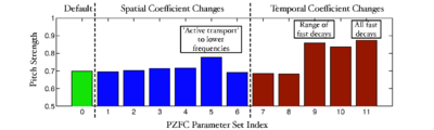
Figure 27 --- Pitch strength measures from SAI profiles generated from a harmonic complex. The PZFC filterbank was used in all cases, and the automatic gain control coefficients of the PZFC were varied.

Figure 28 --- Cochleagrams for the word 'washwater' using the baseline PZFC (top) and PZFC parameter sets 8 and 9 (faster AGC time constants) (middle and bottom). Scaling is as in Figure 16 so that dynamic range can be compared.

Figure 28 shows cochleagrams for the baseline PZFC parameter set (top) and the parameter sets 8 and 9 (middle and bottom) for the word 'washwater' once again. Parameter set 9 produced a considerably higher pitch strength estimate than parameter set 8 for the harmonic complex stimulus. In the cochleagrams, parameter set 9 is seen to apply more compression to the signal than the baseline parameters or parameter set 8. The upper formants of the vowel sounds are now more clearly visible. Although this effect of increased compression has a positive effect on pitch strength, it may in fact degrade the output signal, giving low-level features too much weight relative to high-level ones. In the 'sh' sound, there is considerable activity visible at low frequency, which does not reflect the energy distribution in the input well.

While it is interesting to see that making the AGC of the PZFC react faster has a positive effect in increasing its ability to resolve pitches, it is not immediately clear why this should be the case. Since the effect of fast-acting compression should be to compress glottal-pulses in the input stimulus, one might expect the pitch strength to go down as the speed of the compression was increased. A full study of this effect is beyond the immediate scope of this research, but it is something that I intend to study more fully in the future.

Further work and Conclusions

In this section I have introduced Lyon's pole-zero filter cascade (PZFC) filterbank as an efficient compressive auditory filterbank which can model well the masking data from humans, and compared it to another compressive filterbank, the dynamic compressive gammachirp (dcGC). The PZFC filterbank was implemented in AIM-C and AIM-MAT, using the original implementation by Lyon as a basis. It was tested against dcGC filterbank and the linear and log-compressed gammatone filterbanks in two pitch-strength determination tasks. The PZFC was found to be computationally efficient and to have compression characteristics that enable it to extract pitch from stimuli that have traditionally been challenging to pitch determination algorithms. A number of modifications were made to the automatic gain control (AGC) parameters of the PZFC filterbank to improve its abilities in this regard. These experiments point the way for future work on optimising the PZFC.

The PZFC is an efficient and accurate implementation of an auditory filterbank, and it has the benefit of being based firmly in the fluid dynamics of the cochlea. However, the dcGC filterbank is a better-established filterbank which has been rigorously tested against a variety of psychophysical and physiological data. Currently, the dcGC is better tuned to these data than the PZFC. However, the experiments above demonstrate that it is possible to manipulate parameters of the PZFC AGC to give better performance on certain real-world tasks. Using a similar analysis framework and a wider range of stimuli, it is likely that the PZFC's parameters can be tuned to further improve its performance.

One interesting approach to this problem would be to modify the AGC of the PZFC so that its architecture was more like that of the dcGC. The AGC activity could be shifted so that the state of an AGC stage which takes input from one frequency is used to affect the PZFC filter stage at a lower frequency. This would align the PZFC AGC architecture more closely with models of compression in the cochlea.

The experiments presented in this chapter do not, on their own, justify the use of a compressive filterbank in a machine hearing system. However, they provide an insight into the utility of compressive filterbanks in the processing of stimuli in which the temporal fine structure is important.

A potential continuation of this work would be to use the compressive filterbanks described above in combination with the features generated from the Gaussian mixture model used in the earlier chapters of this thesis. Preliminary experiments to this end, which directly swapped the gammatone filterbank for the PZFC filterbank, led to recognition results which were significantly worse than the results gained with the gammatone filterbank. However the exact parameters of the Gaussian fitting procedure were tuned to the output of a simple gammatone filterbank and these parameters were not modified in the initial experiments. The tuning of these parameters for use with the PZFC and dcGC filterbanks, ideally using a complete search of the parameter space for the Gaussian fitting system, is another potential direction for future work.

While tuning of the AGC circuits of the PZFC, and evaluation of compressive filterbanks with a speech recognition task are probably both worthy of further study, an outstanding opportunity to work with auditory features on a much larger scale suddenly arose in the autumn of 2008. The research team of Dick Lyon at Google had been investigating the use of MFCC features in a large-scale sound effects recognition task, making use of the PAMIR machine learning system which is optimized for use on large datasets. The team was working to extend the model to work with features generated from a version of the auditory image. I was invited to join the team for an internship, working with them on the evaluation of auditory features within the sound effects ranking task.

The system developed at Google was based on the PZFC filterbank and the strobed temporal integration system developed by Dick Lyon and discussed in chapter 3. The speed of the PZFC makes it possible to generate auditory features within a large-scale systems. The efficiency of the filter cascade architecture and the AGC network means that it can provide compressive filtering with not much more computation than a linear gammatone filterbank. This in turn makes it possible for the system to scale to datasets of the size required in Internet search tasks.

Footnotes

Bibliography

Aertsen, A. and Johannesma, P. (1980). “Spectro-temporal receptive fields of auditory neurons in the grassfrog. I. Characterization of tonal and natural stimuli.” Biol. Cybern, 38, p.223-234. [1]
Baker, R.J., Rosen, S. and Darling, A.M. (1998). “An efficient characterisation of human auditory filtering across level and frequency that is also physiologically reasonable”, in Psychophysical and Physiological Advances in Hearing, Palmer, A.R., Rees, A., Summerfield, A.Q. and Meddis, R. editors, p.81-87 (Whurr). [1] [2] [3] [4]
Bilsen, F.A. (2006). “Repetition pitch glide from the step pyramid at Chichen Itza.” J. Acoust. Soc. Am., 120, p.594-. [1]
Carney, L.H., McDuffy, M.J. and Shekhter, I. (1999). “Frequency glides in the impulse responses of auditory-nerve fibers.” J. Acoust. Soc. Am., 105, p.2384-2391. [1]
Cohen, L. (1993). “The scale representation.” IEEE Trans. Sig. Proc., 41, p.3275-3292. [1]
Cooke, M.P. (1993). Modelling auditory processing and organization. (Cambridge University Press). [1]
de Boer, E. (1975). “Synthetic whole-nerve action potentials for the cat.” J. Acoust. Soc. Am., 58, p.1030-. [1]
Flanagan, J.L. and Guttman, N. (1960). “On the pitch of peridic pulses.” J. Acoust. Soc. Am., 32, p.1308-1319. [1]
Fletcher, H. (1940). “Auditory patterns.” Reviews of Modern Physics, 12, p.47-65. [1]
Glasberg, B.R. and Moore, B.C.J. (2000). “Frequency selectivity as a function of level and frequency measured with uniformly exciting notched noise.” J. Acoust. Soc. Am., 108, p.2318-2328. [1] [2] [3]
Handel, S. and Patterson, R.D. (2000). “The perceptual tone/noise ratio of merged, iterated rippled noises with octave, harmonic, and nonharmonic delay ratios.” J. Acoust. Soc. Am., 108, p.692-695. [1]
Huygens, C. (1693). “En envoiant le probleme d'Alhazen en France.” Date-added : 2009-11-27 16:56:45 +0000. Date-modified : 2009-11-27 16:58:28 +0000. Howpublished : printed in Oeuvres Compl{\`e}tes, Vol. 10, edited by Societ{\'y} Hollandaise des Sciences (Nijhoff, Den Haag, 1950), pp.570--571. OriginalCiteRef : huygens:1693. [1]
Irino, T., Walters, T.C. and Patterson, R.D. (2007). “A computational auditory model with a nonlinear cochlea and acoustic scale normalization”, in Proceedings of the 19th International Congress on Acoustics, p.07-003. [1]
Irino, T. and Patterson, R.D. (1997). “A time-domain, level-dependent auditory filter: The gammachirp.” J. Acoust. Soc. Am., 101, p.412-419. [1]
Irino, T. and Patterson, R.D. (2001). “A compressive gammachirp auditory filter for both physiological and psychophysical data.” J. Acoust. Soc. Am., 109, p.2008-2022. [1]
Irino, T. and Patterson, R.D. (2006). “A Dynamic Compressive Gammachirp Auditory Filterbank.” IEEE Transactions on Audio, Speech, and Language Processing, 14, p.2222-2232. [1] [2] [3] [4] [5]
Irino, T. and Unoki, M. (1999). “An analysis/synthesis auditory filterbank based on an IIR implementation of the gammachirp.” J. Acoust. Soc. Jpn, 20, p.397-406. [1]
Ives, D.T. and Patterson, R.D. (2008). “Pitch strength decreases as F0 and harmonic resolution increase in complex tones composed exclusively of high harmonics.” J. Acoust. Soc. Am., 123, p.2670-9. [1] [2] [3] [4] [5]
Johannesma, P. (1972). “The pre-response stimulus ensemble of neurons in the cochlear nucleus.” Pages : 58-69. Booktitle : IPO Symposium on Hearing Theory. IPO, Eindhoven, The Netherlands. OriginalCiteRef : johannesma1972pre. [1]
Kim, D.O., Molnar, C.E. and Matthews, J.W. (1980). “Cochlear mechanics: nonlinear behaviour in two-tone responses as reflected in cochlear-nerve-fibre responses and in ear-canal sound pressure.” J. Acoust. Soc. Am., 67, p.1704-1721. [1]
Krumbholz, K., Patterson, R.D. and Pressnitzer, D. (2000). “The lower limit of pitch as determined by rate discrimination.” J. Acoust. Soc. Am., 108, p.1170-1180. [1]
Lutfi, R.A. and Patterson, R.D. (1984). “On the growth of masking asymmetry with stimulus intensity.” J. Acoust. Soc. Am., 76, p.739-745. [1]
Lyon, R.F. (1996). “The All-Pole Gammatone Filter and Auditory Models.” Journal : unpublished. OriginalCiteRef : Ldraft96. Uri : http://dicklyon.com/tech/Hearing/APGF_Lyon_1996.pdf. [1]
Lyon, R.F. (1997). “All-pole models of auditory filtering”, in Diversity in Auditory Mechanics, E. R. Lewis, S.C. and Lyon, R.F. editors, p.205-211 (World Scientific Publishing, Singapore). [1]
Lyon, R.F. (1998). “Filter cascades as analogs of the cochlea.” Hum. Mov. Sci., , p.3-18. [1] [2] [3] [4]
Lyon, R.F., Katsiamis, A.G. and Drakakis, E.M. (2010). “History and Future of Auditory Filter Models.” OriginalCiteRef : . Booktitle : IEEE International Symposium on Circuits and Systems, 2010. ISCAS 2007. [1] [2] [3] [4]
Lyon, R.F. and Mead, C. (1988). “An analog electronic cochlea.” IEEE Transactions on Acoustics Speech and Signal Processing, 36, p.1119-1134. [1] [2]
Moore, B.C.J. (1995). Hearing. (Academic Press). [1]
Moore, B.C.J. (2003). An Introduction to the Psychology of Hearing. (Academic Press). [1] [2] [3]
Moore, B.C.J., Peters, R.W. and Glasberg, B.R. (1990). “Auditory filter shapes at low center frequencies.” J. Acoust. Soc. Am., 88, p.132-140. [1]
Patterson, R., Holdsworth, J., Nimmo-Smith, I. and Rice, P. (1988). “SVOS final report: The auditory filterbank.” APU report, 2341, p.. [1]
Patterson, R.D., Allerhand, M.H. and Giguère, C. (1995). “Time-domain modeling of peripheral auditory processing: A modular architecture and a software platform.” J. Acoust. Soc. Am., 98, p.1890-1894. [1]
Patterson, R.D., Handel, S., Yost, W.A. and Datta, A.J. (1996). “The relative strength of the tone and noise components in iterated rippled noise.” J. Acoust. Soc. Am., 100, p.3286-3294. [1] [2] [3] [4] [5] [6] [7] [8] [9]
Patterson, R.D., Nimmo-Smith, I., Weber, D.L. and Milroy, R. (1982). “The deterioration of hearing with age: frequency selectivity, the critical ratio, the audiogram, and speech threshold.” J. Acoust. Soc. Am., 72, p.1788-1803. [1]
Patterson, R.D., Unoki, M. and Irino, T. (2003). “Extending the domain of center frequencies for the compressive gammachirp auditory filter.” J. Acoust. Soc. Am., 114, p.1529-1542. [1] [2] [3] [4] [5] [6] [7] [8] [9]
Patterson, R.D., Yost, W.A., Handel, S. and Datta, A.J. (2000). “The perceptual tone/noise ratio of merged iterated rippled noises.” J. Acoust. Soc. Am., 107, p.1578-1588. [1]
Rhode, W.S. and Cooper, N.P. (1993). “Two-tone suppression and distortion production on the basilar membrane in the hook region of the cat and guinea pig cochleae.” Hear. Res., 66, p.31-45. [1]
Rhode, W.S. and Robles, L. (1974). “Evidence from Mössbauer experiments for non-linear vibration in the cochlea.” J. Acoust. Soc. Am., 55, p.588-596. [1]
Rosen, S. and Baker, R.J. (1994). “Characterising auditory filter nonlinearity.” Hear. Res., 73, p.231-243. [1]
Ruggero, M.A., Robles, L. and Rich, N.C. (1992). “Two-tone suppression in the basilar membrane of the cochlea: Mechanical basis of auditory-nerve rate suppression.” J. Neurophysiol., 68, p.1087-1099. [1]
Sachs, M.B. and Kiang, N.Y.S. (1968). “Two-tone inhibition in auditory nerve fibers.” J. Acoust. Soc. Am., 43, p.1120-1128. [1]
Schofield, D. (1985). “Visualisations of speech based on a model of the peripheral auditory system.” Unknown, , p.. [1]
Slaney, M. (1993). An Efficient Implementation of the Patterson-Holdsworth Auditory Filter Bank Apple technical Report. [1] [2]
Unoki, M., Irino, T., Glasberg, B., Moore, B.C. and Patterson, R.D. (2006). “Comparison of the roex and gammachirp filters as representations of the auditory filter.” J. Acoust. Soc. Am., 120, p.1474-1492. [1] [2]
Unoki, M., Irino, T. and Patterson, R.D. (2001). “Improvement of an IIR asymmetric compensation gammachirp filter.” Acoustical Science and Technology, 22, p.426-430. [1] [2] [3]
von Békésy, G. (1960). Experiments in Hearing. (McGraw-Hill). [1]
von Helmholtz, H.L.F. (1875). On the Sensations of Tone as a Physiological Basis for the Theory of Music. (Longmans, Green and Co.). [1]
Wever, E.G. (1949). Theory of hearing. (Wiley). [1]
Yost, W.A. (1996). “Pitch of iterated rippled noise.” J. Acoust. Soc. Am., 100, p.511-518. [1]
Yost, W.A., Patterson, R. and Sheft, S. (1996). “A time domain description for the pitch strength of iterated rippled noise.” J. Acoust. Soc. Am., 99, p.1066-1078. [1] [2]
Yost, W.A., Patterson, R. and Sheft, S. (1998). “The role of the envelope in processing iterated rippled noise.” J. Acoust. Soc. Am., 104, p.2349-2361. [1]
Yost, W.A. and Hill, R. (1979). “Models of the pitch and pitch strength of ripple noise.” J. Acoust. Soc. Am., 66, p.400-. [1]
Zweig, G., Lipes, R. and Pierce, J. (1976). “The cochlear compromise.” J. Acoust. Soc. Am., 59, p.975-. [1]